Calculations in the golden field can be used to study the Fibonacci numbers and other topics related to the golden ratio, notably the geometry of the regular pentagon and higher-dimensional shapes with fivefold symmetry.
Basic arithmetic
Elements of the golden field are those numbers which can be written in the form where and are uniquely determined[3] rational numbers, or in the form where , , and are integers, which can be uniquely reduced to lowest terms, and where is the square root of 5.[4] It is sometimes more convenient instead to use the form where and are rational or the form where , , and are integers, and where is the golden ratio.[5][6]
Converting between these alternative forms is straight-forward: or, in the other direction, .[7]
To add or subtract two numbers, simply add or subtract the components separately:[8]
To find the reciprocal of a number , rationalize the denominator: , where is the algebraic conjugate and is the field norm, as defined below.[9] Explicitly:
To divide two numbers, multiply the first by second's reciprocal:[9]
Conjugation and norm
The numbers and each solve the equation . Each number in has an algebraic conjugate found by swapping these two square roots of 5, i.e., by changing the sign of . The conjugate of is . A rational number is its own conjugate. In general, the conjugate is:[10]
Conjugation in is an involution, , and it preserves the structure of arithmetic: ; ; and .[11] Conjugation is the only ring homomorphism (function preserving the structure of addition and multiplication) from to itself, other than the identity function.[12]
The field trace is the sum of a number and its conjugates (so-called because multiplication by an element in the field can be seen as a kind of linear transformation, the trace of whose matrix is the field trace).[13] The trace of in is :
This is always an (ordinary) rational number.[11]
The field norm is a measure of a number's magnitude, the product of the number and its conjugates.[14] The norm of in is :[11]
This is also always a rational number.[11]
The norm preserves the structure of multiplication, as expected for a concept of magnitude. The norm of a product is the product of norms, ; and the norm of a quotient is the quotient of the norms, . A number and its conjugate have the same norm, ;[11]
In Galois theory, the golden field can be considered more abstractly as the set of all numbers , where and are both rational, and all that is known of is that it satisfies the equation . There are two ways to embed this set in the real numbers: by mapping to the positive square root or alternatively by mapping to the negative square root . Conjugation exchanges these two embeddings. The Galois group of the golden field is thus the group with two elements, namely the identity and an element which is its own inverse.[14]
Golden integers
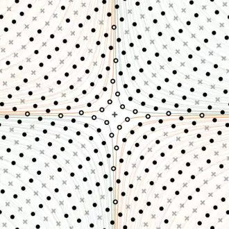
One convenient way to plot is as a lattice, using the number as the horizontal coordinate and its conjugate as the vertical coordinate. Then numbers with the same norm lie on hyperbolas (orange and green lines).
The ring of integers of the golden field, , sometimes called the golden integers,[15] is the subset of algebraic integers in the field, meaning those elements whose minimal polynomial over has integer coefficients. These are the set of numbers in whose norm is an integer. The numbers and form an integral basis for the ring, meaning every number in the ring can be written in the form where and are ordinary integers.[16] Alternately, elements of can be written in the form , where and have the same parity.[17] Like any ring, is closed under addition and multiplication.
The set of all norms of golden integers includes every number for ordinary integers and . These are precisely the integers whose prime factors which are congruent to modulo occur with even exponents. The first several non-negative integer norms are:[18]
The golden integer is called zero, and is the only element of with norm .[19]
A unit is an algebraic integer whose multiplicative inverse is also an algebraic integer, which happens when its norm is . The units of , when written in the form , have coefficients which solve the generalized Pell's equation. The fundamental unit is the golden ratio and the other units are its positive and negative powers, , for any integer .[3] Some powers of are:
In general , where is the th Fibonacci number.[20][8] The units form a group under multiplication, which can be decomposed as the direct product of a cyclic group of order 2 and an infinite cyclic group, respectively generated by and .
Two golden integers are associates if their quotient in is a unit; that is, two golden integers and are associates if for some integer . Associateness is an equivalence relation. Associates have the same norm, up to sign: . However, not all elements whose norm has the same absolute value are associates; in particular, any golden prime and its conjugate have the same norm, but are associates if and only if they are associated either with or with an ordinary prime.
Golden integer units (hollow circles) and primes (filled circles), along with zero (+) and composite numbers (×)[21]
The prime elements of the ring, analogous to prime numbers among the integers, are of three types: , integer primes of the form where is an integer, and the factors of integer primes of the form (a pair of conjugates).[22] For example, , , and are primes, but is composite. Any of these is an associate of additional primes found by multiplying it by a unit; for example is also prime because is a unit.
Like all Euclidean domains, the ring shares many properties with the ring of integers. In particular, it is a principal ideal domain, and it satisfies a form of the fundamental theorem of arithmetic: every element of can be written as a product of prime elements multiplied by a unit, and this factorization is unique up to the order of the factors and the replacement of any prime factor by an associate prime (which changes the unit factor accordingly).
In the table below, positive golden integers have been arranged into rows, with one representative chosen for each class of associates (here the representative is the positive element in the class for which is a minimum).
Rep.
Norm
Trace
Factorization
Positive associates
zero
unit
, , , ; , , ,
prime
, , ; , ,
prime
, , ; , ,
prime
, , ; , ,
prime
, , ; , ,
prime
, , ; ,
, , ; , ,
prime
, , ; , ,
prime
, , ; , ,
, , ; , ,
, , ; , ,
prime
, , ; , ,
prime
, , ; , ,
prime
, , ; , ,
prime
, , ; , ,
, , ; , ,
prime
, , ; , ,
prime
, , ; , ,
, , ; , ,
, , ; , ,
, , ; , ,
prime
, , ; , ,
, , ; , ,
, , ; , ,
prime
, , ; , ,
prime
, , ; , ,
Show/hide more rows
Matrix representation
is a two-dimensional vector space over , and multiplication by any element of is a linear transformation of that vector space. Given an ordered basis of , each number in can be associated to the corresponding transformation matrix in that basis. This defines a field isomorphism (a structure-preserving bijective map) from to the space of square matrices with rational entries spanned by the identity matrix, the image of the number , and a matrix , the image of .[25] Thus arithmetic of numbers in can be alternately represented by the arithmetic of such matrices.[26] In this context, the number is represented by the matrix .[27] A convenient choice of basis for is , in terms of which is a symmetric matrix:[28]
The adjugate matrix represents the algebraic conjugate , the matrix (satisfying ) represents ,[29] and the adjugate of an arbitrary element , which we will denote , represents the number :
Every matrix , except for the zero matrix, is invertible, and its inverse represents the multiplicative inverse in .[30]
If is an element of , with conjugate , then the matrix has the numbers and as its eigenvalues. Its trace is . Its determinant is . The characteristic polynomial of is , which is the minimal polynomial of and whenever is not zero. These properties are shared by the adjugate matrix . Their product is .[26][25]
These matrices have especially been studied in the context of the Fibonacci numbers and Lucas numbers, which appear as the entries of and , respectively:
Powers of are sometimes called Fibonacci matrices.[31]
Every matrix of the form has eigenvectors which point along the directions and . When numbers in are plotted, as above, in a coordinate system where their values as real numbers are the horizontal axis and the values of their conjugates are the vertical axis, the eigenvectors point along those two axes. (Zero is the only number directly on either axis.) The matrices for integer , representing units, and more generally any matrices with and determinant , are squeeze mappings, which stretch the plane along one axis and squish it along the other, fixing hyperbolas of constant norm. The matrices and more generally matrices with and determinant , are the composition of a squeeze mapping and a vertical reflection. The negative identity matrix is a point reflection across the origin. In general any other matrix can be decomposed as the product of a squeeze mapping, possibly a reflection, and a uniform scaling by the square root of the absolute value of its determinant.
Any positive element of the golden field can be written as a generalized type of continued fraction, in which the partial quotients are sums of non-negative powers of .[34]
Fibonacci numbers
The Lucas and Fibonacci numbers are components of φn when written in terms of 1/2 and 1/2√5.[35]
is a useful number system to use when studying the Fibonacci numbers and the Lucas numbers. These number sequences are usually defined by recurrence relations similar to the one satisfied by the powers of and :
Both sequences can be consistently extended to negative integer indices by following the same recurrence in the negative direction. They satisfy the identities[37]
The Fibonacci and Lucas numbers can alternately be expressed as the components and when a power of the golden ratio or its conjugate is written in the form :[38]
Binet's formula for Fibonacci numbers plotted in the lattice of golden integers
The expression of the Fibonacci numbers in terms of is called Binet's formula:[39]
The powers of or , when written in the form , can be expressed in terms of just Fibonacci numbers,[20]
Powers of or times can be expressed in terms of just Lucas numbers,
Statements about golden integers can be recast as statements about the Fibonacci or Lucas numbers; for example, that every power of is a unit of , , when expanded, becomes Cassini's identity, and likewise becomes the analogous identity about Lucas numbers,
The numbers and are the roots of the quadratic polynomial . This is the minimal polynomial for for any non-zero integer .[40] The quadratic polynomial is the minimal polynomial for .[41]
In the limit, consecutive Fibonacci or Lucas numbers approach a ratio of , and the ratio of Lucas to Fibonacci numbers approaches :[4]
Theorems about the Fibonacci numbers – for example, divisibility properties such as if divides then divides – can be conveniently proven using .[42]
Relation to fivefold symmetry
The golden ratio is the ratio between the lengths of a diagonal and a side of a regular pentagon, so the golden field and golden integers feature prominently in the metrical geometry of the regular pentagon and its symmetry system, as well as higher-dimensional objects and symmetries involving five-fold symmetry.
Euclidean plane
The golden ratio is related to the fifth roots of unity.
Let be the 5th root of unity, a complex number of unit absolute value spaced of a full turn from around the unit circle, satisfying . Then the fifth cyclotomic field is the field extension of the rational numbers formed by adjoining (or equivalently, adjoining any of , or ). Elements of are numbers of the form , with rational coefficients. is of degree four over the rational numbers: any four of the five roots are linearly independent over , but all five sum to zero. However, is only of degree two over ,
where the conjugate . The elements of can alternately be represented as , where and are elements of :
Conversely, is a subfield of . For any primitive root of unity , the maximal real subfield of the cyclotomic field is the field ; see Minimal polynomial of . In our case , , so the maximal real subfield of is .[43]
Angles of and thus have golden rational cosines but their sines are the square roots of golden rational numbers.[44]
The numbers and are conjugates with norm . These are the squared Euclidean lengths of the diagonal and side, respectively, of a regular pentagon with unit circumradius.
The 600-cell is a regular 4-polytope with 120 vertices, 720 edges, 1200 triangular faces, and 600 tetrahedral cells. It has kaleidoscopic symmetry generated by four mirrors which can be conveniently oriented as , , , and . Then the 120 vertices have golden-integer coordinates: arbitrary permutations of and with an even number of minus signs, with an odd number of minus signs, and .[46][47]
Higher dimensions
The icosians are a special set of quaternions that are used in a construction of the E8 lattice. Each component of an icosian always belongs to the golden field.[48] The icosians of unit norm are the vertices of a 600-cell.[47]
Quasiperiodicity
The Fibonacci chain, a one-dimensional quasicrystal, constructed by the cut-and-project method
^The expression is pronounced "the rational numbers adjoin the square root of five", or, more concisely, "Q adjoin root five". See Trifković 2013, p. 6.
^ abLiba & Ilany 2023, p. 15; Fontaine & Hurley 2011 also mention the isomorphism between the real subfield of the cyclotomic field and the arithmetic of matrices spanned by and , which they call the silver matrices and . Méndez-Delgadillo, Lam-Estrada & Maldonado-Ramírez 2015 work with the basis , relative to which the matrix represents :
In this basis, the golden ratio is represented by a matrix : This is the same idea as using the matrices and : arithmetic of these matrices is likewise isomorphic to arithmetic in , and the eigenvalues, characteristic polynomial, trace, and determinant are the same in any basis. However, the eigenvectors are and rather than and .
^ abRotman 2017, p. 456 ff. describes this for finite-dimensional field extensions in general.
^Our matrix , or the mirrored variant , is commonly denoted or in work about the Fibonacci numbers. See Gould 1981 for a survey in that context. Here we use the symbol for consistency with the symbol and to avoid confusion with the rational numbers , which are also often denoted . Liba & Ilany 2023, p. 15 also use the symbol , and call this the "golden matrix".
^For , which is its own conjugate, the polynomial is not minimal.
^Because, as described in § Conjugation and norm, for any in . In this case, , , , and .
^Dodd 1983, § 9.4 "Divisibility Properties of the Fibonacci Numbers", pp. 119–126 proves this and various related results. See also Carlitz 1964.
^More generally, for any odd prime , the field is a subfield of . Moreover, by the Kronecker–Weber theorem, every abelian extension of the rationals is contained in some cyclotomic field. See Ireland & Rosen 1990, pp. 199–200.
Bradie, Brian (2002). "Exact Values for the Sine and Cosine of Multiples of – A Geometric Approach". Classroom Capsules. The College Mathematics Journal. 33 (4): 318–319. doi:10.1080/07468342.2002.11921960.
Dimitrov, Vassil S.; Cosklev, T. V.; Bonevsky, B. (1995). "Number theoretic transforms over the golden section quadratic field". IEEE Transactions on Signal Processing. 43 (8): 1790–1797. doi:10.1109/78.403338.
Hunt, Bruce (1996). "The 27 lines on a cubic surface". The Geometry of some special Arithmetic Quotients. Berlin: Springer. doi:10.1007/BFb0094404. ISBN 3-540-61795-7.
Liba, Opher; Ilany, Bat-Sheva (2023). From the Golden Rectangle to the Fibonacci Sequences. Contributions by Nativ, Isaac. Cham: Springer. doi:10.1007/978-3-030-97600-2 (inactive 19 Jul 2025). ISBN 978-3-030-97599-9.{{cite book}}: CS1 maint: DOI inactive as of July 2025 (link) Originally published as ממלבן הזהב לסדרות פיבונאצי. Tel Aviv: Mofet Institute. 2019.
Pleasants, Peter A. B. (2002). "Lines and Planes in 2- and 3-Dimensional Quasicrystals". In Kramer, Peter; Papadopolos, Zorka (eds.). Coverings of Discrete Quasiperiodic Sets. Berlin: Springer. pp. 185–225. doi:10.1007/3-540-45805-0_6. ISBN 3-540-43241-8.
Polo-Blanco, Irene; Top, Jaap (2009). "A remark on parameterizing nonsingular cubic surfaces". Computer Aided Geometric Design. 26 (8): 842–849. doi:10.1016/j.cagd.2009.06.001.
Rotman, Joseph J. (2017) [2002]. "Algebraic Integers". Advanced Modern Algebra. Vol. 2. American Mathematical Society. §C-5.3.2, pp. 455–467. ISBN 978-1-4704-2311-7.


+(a_{2}+b_{2}\varphi )&=(a_{1}+a_{2})+(b_{1}+b_{2})\varphi .\end{aligned}}}](./_assets_/1cd574aaedc320876989bdcfd331fdb011cc2fa4.svg)
(a_{2}+b_{2}\varphi )&=(a_{1}a_{2}+b_{1}b_{2})+(a_{1}b_{2}+b_{1}a_{2}+b_{1}b_{2})\varphi .\end{aligned}}}](./_assets_/28934f71c47f98b29cfaacc1f4ef509a633590ce.svg)


![{\displaystyle {\begin{aligned}{\frac {1}{a+b{\sqrt {5}}}}&={\frac {1}{a+b{\sqrt {5}}}}\cdot {\frac {a-b{\sqrt {5}}}{a-b{\sqrt {5}}}}={\frac {a}{a^{2}-5b^{2}}}-{\frac {b}{a^{2}-5b^{2}}}{\sqrt {5}},\\[3mu]{\frac {1}{a+b\varphi }}&={\frac {1}{a+b\varphi }}\cdot {\frac {a+b-b\varphi }{a+b-b\varphi }}={\frac {a+b}{a^{2}+ab-b^{2}}}-{\frac {b}{a^{2}+ab-b^{2}}}\varphi .\end{aligned}}}](./_assets_/8b14521b41cd4243060fd7b84d6459ef13c53372.svg)
![{\displaystyle {\begin{aligned}{\frac {a_{1}+b_{1}{\sqrt {5}}}{a_{2}+b_{2}{\sqrt {5}}}}&={\frac {a_{1}a_{2}-5b_{1}b_{2}}{a_{2}^{2}-5b_{2}^{2}}}+{\frac {-a_{1}b_{2}+b_{1}a_{2}}{a_{2}^{2}-5b_{2}^{2}}}{\sqrt {5}},\\[6mu]{\frac {a_{1}+b_{1}\varphi }{a_{2}+b_{2}\varphi }}&={\frac {a_{1}a_{2}+a_{1}b_{2}-b_{1}b_{2}}{a_{2}^{2}+a_{2}b_{2}-b_{2}^{2}}}+{\frac {-a_{1}b_{2}+b_{1}a_{2}}{a_{2}^{2}+a_{2}b_{2}-b_{2}^{2}}}\varphi .\end{aligned}}}](./_assets_/752ff01ca8b80a40f879efd3aad40a0ee9eaa427.svg)


![{\displaystyle {\begin{aligned}{\overline {a+b{\sqrt {5}}}}&=a-b{\sqrt {5}},\\[3mu]{\overline {a+b\varphi }}&=a+b{\overline {\varphi }}=(a+b)-b\varphi .\end{aligned}}}](./_assets_/6325a917020f6d0d66f8816ec4383650cb2bfa5a.svg)


![{\displaystyle {\begin{aligned}\mathrm {Tr} {\bigl (}a+b{\sqrt {5}}~\!{\bigr )}&={\bigl (}a+b{\sqrt {5}}~\!{\bigr )}+{\bigl (}a-b{\sqrt {5}}~\!{\bigr )}=2a,\\[3mu]\mathrm {Tr} (a+b\varphi )&=(a+b\varphi )+(a+b-b\varphi )=2a+b.\end{aligned}}}](./_assets_/95538af7c28a6c482a5a7bdd71dae1e3cd1b2b01.svg)

![{\displaystyle {\begin{aligned}\mathrm {N} {\bigl (}a+b{\sqrt {5}}~\!{\bigr )}&=a^{2}-5b^{2},\\[3mu]\mathrm {N} (a+b\varphi )&=a^{2}+ab-b^{2}.\end{aligned}}}](./_assets_/a70f81ed8b29a5db21039b5c582d5b2f1a7d624a.svg)


![{\displaystyle \mathbb {Z} [\varphi ]}](./_assets_/14f984c2710477c64fca0f16a71928134bdb8201.svg)




![{\displaystyle {\begin{aligned}\mathbf {\Phi } ^{n}&=F_{n-1}\mathbf {I} +F_{n}\mathbf {\Phi } ={\begin{bmatrix}F_{n-1}&F_{n}~\\F_{n}~&F_{n+1}\end{bmatrix}},&\mathrm {Tr} (\mathbf {\Phi } ^{n})&=L_{n},\\[8mu]\mathbf {\Phi } ^{n}\mathbf {R} &=L_{n-1}\mathbf {I} +L_{n}\mathbf {\Phi } ={\begin{bmatrix}L_{n-1}&L_{n}~\\L_{n}~&L_{n+1}\end{bmatrix}},&\mathrm {Tr} (\mathbf {\Phi } ^{n}\mathbf {R} )&=5F_{n}.\end{aligned}}}](./_assets_/2dd51dde47e4538678151aef8d0ee0cc757d387f.svg)


![{\displaystyle {\begin{aligned}F_{0}&=0,&F_{1}&=1,&F_{n+1}&=F_{n}+F_{n-1},\\[3mu]L_{0}&=2,&L_{1}&=1,&L_{n+1}&=L_{n}+L_{n-1},\\[3mu]\varphi ^{0}&=1,&\varphi ^{1}&=\varphi ,&\varphi ^{n+1}&=\varphi ^{n}+\varphi ^{n-1},\\[3mu]{\overline {\varphi }}^{0}&=1,&{\overline {\varphi }}^{1}&={\overline {\varphi }},&{\overline {\varphi }}^{n+1}&={\overline {\varphi }}^{n}+{\overline {\varphi }}^{n-1}.\end{aligned}}}](./_assets_/e32f8fd4ca2348d7be1838bd4b36a0f03055d9ab.svg)


![{\displaystyle {\begin{aligned}\varphi ^{n}&={\tfrac {1}{2}}L_{n}+{\tfrac {1}{2}}F_{n}{\sqrt {5}},\\[3mu]{\overline {\varphi }}^{n}&={\tfrac {1}{2}}L_{n}-{\tfrac {1}{2}}F_{n}{\sqrt {5}}.\end{aligned}}}](./_assets_/c2bbbfe703b69da77f7aff389c191ac65a070edb.svg)

![{\displaystyle {\begin{aligned}F_{n}&={\frac {\varphi ^{n}-{\overline {\varphi }}^{n}}{\varphi -{\overline {\varphi }}}}={\frac {\varphi ^{n}-{\overline {\varphi }}^{n}}{\sqrt {5}}}={\frac {\mathrm {Tr} {\bigl (}\varphi ^{n}{\sqrt {5}}~\!{\bigr )}}{5}},\\[5mu]L_{n}&={\frac {\varphi ^{n}+{\overline {\varphi }}^{n}}{\varphi +{\overline {\varphi }}}}=\varphi ^{n}+{\overline {\varphi }}^{n}=\mathrm {Tr} {\left(\varphi ^{n}\right)}.\end{aligned}}}](./_assets_/217e56336961764d72a1c8555ce22cf36823d2d0.svg)
![{\displaystyle {\begin{aligned}\varphi ^{n}&=F_{n-1}+F_{n}\varphi ,\\[3mu]{\overline {\varphi }}^{n}&=F_{n-1}+F_{n}{\overline {\varphi }}=F_{n+1}-F_{n}\varphi .\end{aligned}}}](./_assets_/6b6910616120e88b54f6c9a639cc313d489c6b1f.svg)
![{\displaystyle {\begin{aligned}\varphi ^{n}{\sqrt {5}}&=L_{n-1}+L_{n}\varphi ,\\[3mu]{\overline {\varphi }}^{n}{\sqrt {5}}&=-L_{n-1}-L_{n}{\overline {\varphi }}=-L_{n+1}+L_{n}\varphi .\end{aligned}}}](./_assets_/fab50d820b41547cf39e18f3c41713b1caf7c029.svg)


(-L_{n+1}+L_{n}\varphi )&=L_{n}^{2}-L_{n-1}L_{n+1}=(-1)^{n}5.\end{aligned}}}](./_assets_/334976ac65c89580b59df03c62e0b9ed6c03ce8e.svg)


![{\displaystyle {\begin{aligned}x^{5}-1&=(x-1){\bigl (}x^{4}+x^{3}+x^{2}+x+1{\bigr )}\\[2mu]&=(x-1){\bigl (}x^{2}+{\overline {\varphi }}x+1{\bigr )}{\bigl (}x^{2}+\varphi x+1{\bigr )}\\[2mu]&=(x-1){\bigl (}x-\zeta {\bigr )}{\bigl (}x-\zeta ^{4}{\bigr )}{\bigl (}x-\zeta ^{2}{\bigr )}{\bigl (}x-\zeta ^{3}{\bigr )},\end{aligned}}}](./_assets_/c7f6c061fcfae378f0e98e902dace3e4b3733b39.svg)


![{\displaystyle {\begin{aligned}&a_{0}+a_{1}\zeta +a_{2}\zeta ^{2}+a_{3}\zeta ^{3}+a_{4}\zeta ^{4}\\[3mu]&\qquad ={\bigl (}a_{0}-a_{2}+{\overline {\varphi }}a_{3}-{\overline {\varphi }}a_{4}{\bigr )}+{\bigl (}a_{1}-{\overline {\varphi }}a_{2}+{\overline {\varphi }}a_{3}-a_{4}{\bigr )}\zeta .\end{aligned}}}](./_assets_/5d2ce44f25d3a285e8f30ced7cd750e1b31433cc.svg)


![{\displaystyle {\begin{alignedat}{3}\zeta &={\tfrac {1}{2}}{\bigl (}{-{\overline {\varphi }}}+{\textstyle {\sqrt {\,{\overline {\varphi }}{}^{2}-4}}}~\!{\bigr )}&{}=-{\tfrac {1}{2}}{\overline {\varphi }}+{\tfrac {1}{2}}{\sqrt {-2-\varphi }},\\[6mu]\zeta ^{2}&={\tfrac {1}{2}}{\bigl (}{-\varphi }+{\textstyle {\sqrt {\varphi {}^{2}-4}}}~\!{\bigr )}&{}=-{\tfrac {1}{2}}\varphi +{\textstyle {\tfrac {1}{2}}{\sqrt {-2-{\overline {\varphi }}}}}.\end{alignedat}}}](./_assets_/0f715c0b2bd051ef5a85b606e49c9dfc6e4b3649.svg)


![{\displaystyle {\begin{aligned}\cos {\tfrac {2}{5}}\pi &=-{\tfrac {1}{2}}{\overline {\varphi }},&\sin {\tfrac {2}{5}}\pi &={\tfrac {1}{2}}{\sqrt {2+\varphi }},\\[6mu]\cos {\tfrac {4}{5}}\pi &=-{\tfrac {1}{2}}\varphi ,&\sin {\tfrac {4}{5}}\pi &={\tfrac {1}{2}}{\textstyle {\sqrt {2+{\overline {\varphi }}}}}.\end{aligned}}}](./_assets_/476a0abef995df9845079dcdde68780c1dc44e82.svg)


![{\displaystyle [5,3,3]}](./_assets_/d5a43aec7a9e2758707d07cddc99e36f91a9d13f.svg)


![{\displaystyle \mathbf {Q} [{\sqrt {n}}~\!]}](./_assets_/102d8fc8d9fd2f2fb8ca4d3ad7a38856f97455c8.svg)
![{\displaystyle S[5,1]}](./_assets_/eade34606e86acdfe69c64e2480527f95423075a.svg)
![{\displaystyle S[5,2]}](./_assets_/37d28870ad388737204edcc2a7b83baa9df3a050.svg)


![{\displaystyle {\bigl [}{\begin{smallmatrix}1&1\\1&0\end{smallmatrix}}{\bigr ]}}](./_assets_/d6bd41b1df6016696ca8fd637422f98feb58aaf2.svg)


